Long Short Term Memory (LSTM)
The recurrent neural network model used to perform this task is a long short-term memory (LSTM) network. This type of network is preferred over simple recurrent networks (SNR) as it can avoid both vanishing and exploding gradients associated with SNRs. LSTM networks are able to learn long range dependencies by using a combination of three internal neural networks: forget, input and output gates. Each of these gates is a feed forward network layer which are made of weights that the network will learn, as well as an activation function (Lane et al. 2019).
The forget gate is used to determine a ratio between 0 and 1 for each cell unit \(C_{t-1}\). If the ratio is close to zero, the previous value of the corresponding cell unit will be mostly forgotten. Whereas, a ratio close to one will mostly preserved the previous value. The torch.nn.LSTM() function from PyTorch computes the forget gate function using the following formula:
The activation function for this gate is a sigmoid activation function, which outputs values between 0 and 1 for each cell unit.
The next step is to decide what new information we will add to the cell unit (i.e. update values). The update values \((g)\) are between -1 and +1, which are computed using tanh, and the input gate \((i)\) is used to determine the ratios by which these update values will be multiplied before being added to the current cell unit values. This is represented by the following mathematical formulas:
The cell unit value is then updated by combining the input gate (\(i_t\)) and tanh (\(g_t\)) and doing an element-wise multiplication between the forget gate (\(f_t\)) and the sum product of this, as shown by the following formula:
The final output gate \((o)\) computes the ratios by which tanh of the cell unit values will be multiplied with the aim of producing the next hidden unit values with the following mathematical formula:
This type of network allows the cell unit to specialise, with some changing their values regularly while others preserving their state for many iterations.
Bidirectional LSTM (bi-LSTM)
A common variation of the LSTM are bidirectional LSTMs where the input is presented forwards and backwards to two separate recurrent networks, both of which are connected to the same output layer (Graves & Schmidhuber 2005). Bi-LSTM networks provide additional context to the sequence and can improve model performance in classification tasks.
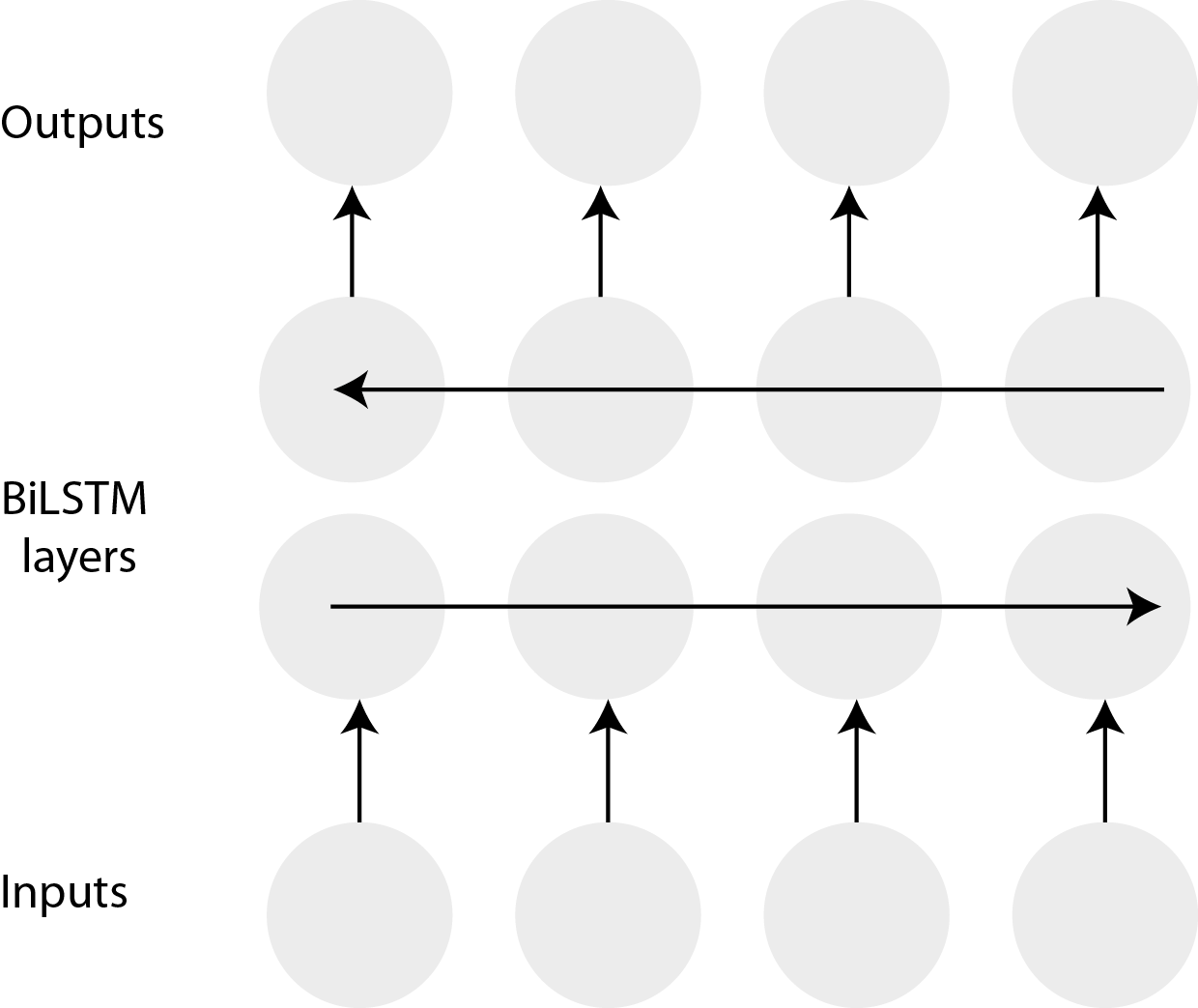
Fig. 1 Figure 1: A bi-LSTM. Source: (Pointer 2019)